44 format data labels pane excel

Excel 2016 Tutorial Formatting Data Labels Microsoft Training Lesson Jan 12, 2016 ... FREE Course! Click: about Formatting Data Labels in Microsoft Excel at . Microsoft 365 Roadmap | Microsoft 365 You can create PivotTables in Excel that are connected to datasets stored in Power BI with a few clicks. Doing this allows you get the best of both PivotTables and Power BI. Calculate, summarize, and analyze your data with PivotTables from your secure Power BI datasets. More info. Feature ID: 63806; Added to Roadmap: 05/21/2020; Last Modified ...

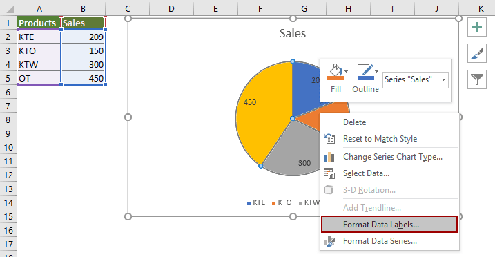
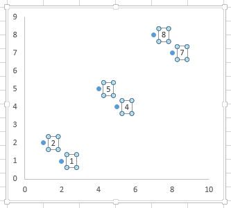
Scatter plot excel with labels - fjahqr.sanitaer-friedhelm.de Sep 06, 2022 · A drop-down appears. Click on the Format Data Labels option. Step 4: Format Data Labels dialogue box appears. Under the Label Options, check the box Value from Cells . Step 5: Data Label Range dialogue-box appears. Right click any data point and click 'Add data labels and Excel will pick one of the

Format data labels pane excel

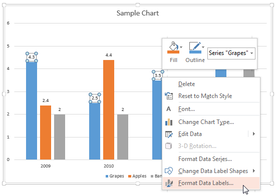
How to Add and Format Data Labels | Learning Excel - YouTube Jan 13, 2022 ... How to Add and Format Data Labels | Learning Excel#How_to_Add_and_Format_Data_Labels. How to Make Excel Clustered Stacked Column Chart - Data Fix Oct 11, 2022 · A) Data in a Summary Grid - Rearrange the Excel data, then make a chart; B) Data in Detail Rows - Make a Pivot Table & Pivot Chart; C) Data in a Summary Grid - Save Time with Excel Add-In; Clustered Stacked Chart Example. In the examples shown below, there are . 2 years of data; 4 seasons of sales amounts each year; 4 different regions How to Format Data Labels in Excel (with Easy Steps) - ExcelDemy Aug 2, 2022 ... Step-by-Step Procedure to Format Data Labels in Excel · Step 1: Create Chart · Step 2: Add Data Labels to Chart · Step 3: Modify Fill and Line of ...

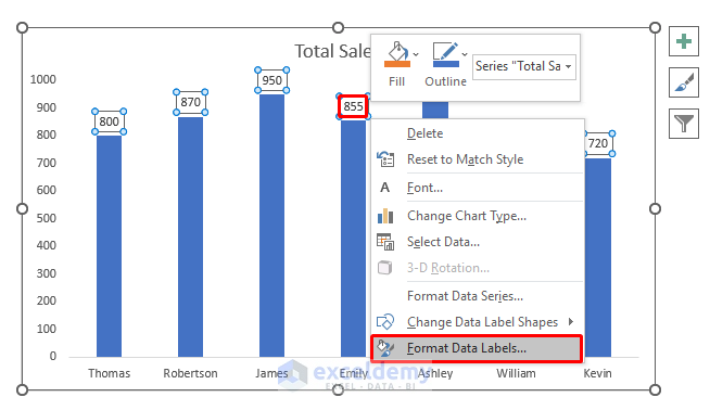
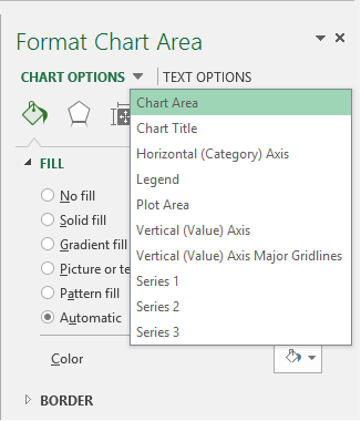
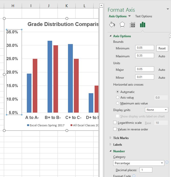
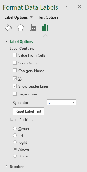
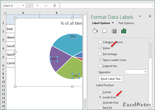
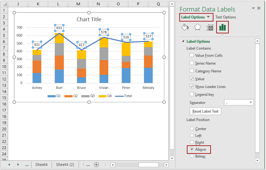
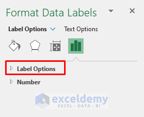
Format data labels pane excel. Change the format of data labels in a chart - Microsoft Support Format Data Labels task pane. To get there, after adding your data labels, select the data label to format, and then click ; Chart Elements Chart Elements button ... Pie Chart in Excel - Inserting, Formatting, Filters, Data Labels Dec 29, 2021 · The chart would consider the absolute ( positive ) value for any negative value in the data ; The total of percentages of the data point in the pie chart would be 100% in all cases. Consequently, we can add Data Labels on the pie chart to show the numerical values of the data points. We can use Pie Charts to represent: Change axis labels in a chart - support.microsoft.com Your chart uses text from its source data for these axis labels. Don't confuse the horizontal axis labels—Qtr 1, Qtr 2, Qtr 3, and Qtr 4, as shown below, with the legend labels below them—East Asia Sales 2009 and East Asia Sales 2010. Change the text of the labels. Click each cell in the worksheet that contains the label text you want to ... Formatting Data Labels Ribbon: On the Series tab, in the Properties group, open the Data Labels drop-down menu and select More Data Labels Options to open the Format Labels dialog box ...

Excel data doesn't retain formatting in mail merge - Office Mar 31, 2022 · Then, select Format, and then select Format Cells. Select Number tab. Under Category, select Text, and then select OK. Save the data source. Then, continue with the mail merge operation in Word. References. Date, Phone Number, and Currency fields are merged incorrectly when you use an Access or Excel data source in Word Excel Charts - Aesthetic Data Labels - Tutorialspoint Step 1 − Click twice any data label you want to format. Step 2 − Right-click that data label and then click Format Data Label. Alternatively, you can also ... Creating a chart with dynamic labels - Microsoft Excel 365 Add the labels values from the cells · For all labels: Right-click on any data label and select Format Data Labels... in the popup menu: · For the specific label: ... How to Create a Pareto Chart in Excel – Automate Excel Step #7: Add data labels. It’s time to add data labels for both the data series (Right-click > Add Data Labels). As you may have noticed, the labels for the Pareto line look a bit messy, so let’s place them right above the line. To reposition the labels, right-click on the data labels for Series “Cumulative %” and choose “Format Data ...

Add or remove data labels in a chart - Microsoft Support You can also right-click the selected label or labels on the chart, and then click Format Data Label or Format Data Labels. Click Label Options if it's not ... Excel 2019 & 365 Tutorial Formatting Data Labels Microsoft Training Sep 3, 2019 ... FREE Course! Click: Learn about Formatting Data Labels in Microsoft Excel at . Format Data Labels in Excel- Instructions - TeachUcomp, Inc. Nov 14, 2019 ... To format data labels in Excel, choose the set of data labels to format. To do this, click the “Format” tab within the “Chart Tools” contextual ... How to Format Data Labels in Excel (with Easy Steps) - ExcelDemy Aug 2, 2022 ... Step-by-Step Procedure to Format Data Labels in Excel · Step 1: Create Chart · Step 2: Add Data Labels to Chart · Step 3: Modify Fill and Line of ...

Cannot change the data label number formatting in ...

How to Make Excel Clustered Stacked Column Chart - Data Fix Oct 11, 2022 · A) Data in a Summary Grid - Rearrange the Excel data, then make a chart; B) Data in Detail Rows - Make a Pivot Table & Pivot Chart; C) Data in a Summary Grid - Save Time with Excel Add-In; Clustered Stacked Chart Example. In the examples shown below, there are . 2 years of data; 4 seasons of sales amounts each year; 4 different regions

How to show percentages on three different charts in Excel ...

How to Add and Format Data Labels | Learning Excel - YouTube Jan 13, 2022 ... How to Add and Format Data Labels | Learning Excel#How_to_Add_and_Format_Data_Labels.

Format Data Label Options in PowerPoint 2013 for Windows

How to improve or conditionally format data labels in Power ...

How to Make Pie Chart with Labels both Inside and Outside ...

Creating Pie Chart and Adding/Formatting Data Labels (Excel)

Change the format of data labels in a chart

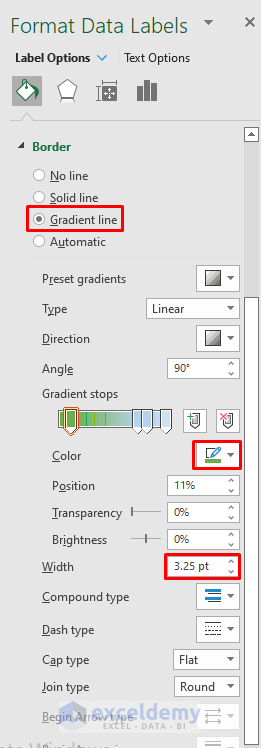
How to Format Data Labels in Excel (with Easy Steps) - ExcelDemy

How to Create a Bar Chart With Labels Inside Bars in Excel

Add a Data Callout Label to Charts in Excel 2013 – Software ...

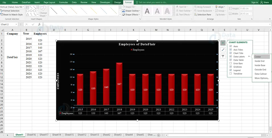
Elements and Options Of Chart in Excel - DataFlair

How to Rotate Data Labels in Excel (2 Simple Methods)

Change the format of data labels in a chart

Adding rich data labels to charts in Excel 2013 | Microsoft ...

Excel Charts - Formatting

Change the format of data labels in a chart

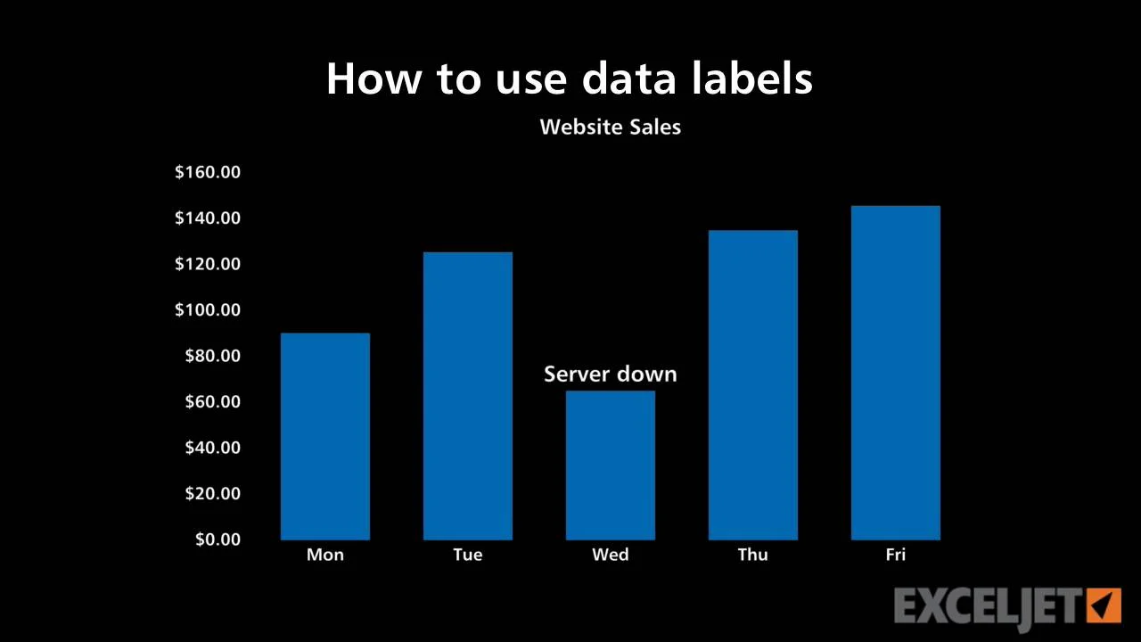
How to use data labels

How to show percentages on three different charts in Excel ...

Dynamically Label Excel Chart Series Lines • My Online ...

Apply Custom Data Labels to Charted Points - Peltier Tech

Change the format of data labels in a chart

Change the format of data labels in a chart

Excel 2016 In Practice Guided Project 3-3 Instructions

How to show percentage in pie chart in Excel?

4.2 Formatting Charts – Beginning Excel, First Edition

How to add and customize chart data labels

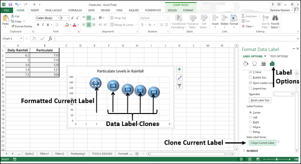
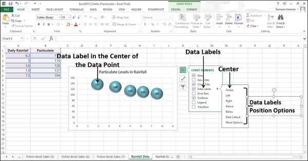
Excel Charts - Aesthetic Data Labels

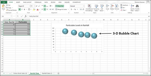
Excel Charts - Aesthetic Data Labels

Is it possible to adjust the data label text box dimension in ...

How to Customize Your Excel Pivot Chart Data Labels - dummies

Apply Custom Data Labels to Charted Points - Peltier Tech

Adding rich data labels to charts in Excel 2013 | Microsoft ...

Using the CONCAT function to create custom data labels for an ...

CIS Ch3 Excel Flashcards | Quizlet

How to add a text label in the chart of MS Excel - Quora

How to Add Data Labels to an Excel 2010 Chart - dummies

Add or remove data labels in a chart

Change the format of data labels in a chart

How to Make Pie Chart with Labels both Inside and Outside ...

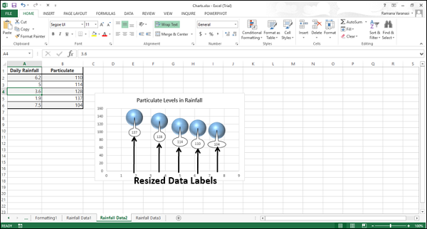
Excel Charts - Aesthetic Data Labels

Excel Charts - Aesthetic Data Labels

Format Data Labels in Excel- Instructions - TeachUcomp, Inc.

How to add total labels to stacked column chart in Excel?

How to Move Data Labels In Excel Chart (2 Easy Methods)

Share :